*** COLLATZ BREAKTHRU *** (“2”)

💡 💡 💡 ❗ ❗ ❗ ⭐ ⭐ ⭐ 😮 hi all, am coding/ working late on a weeknite which is uncommon for me these days but was fueled by some flashes of inspiration. was dinking around with some engaging/ fresh ideas and then came up and ran into this apparent ***BREAKTHRU*** so am not waiting to share it! (carpe diem!)

this code generates a random hard trajectory with glide length over 100, and then computes the 2^nd (integer/ sequence) “derivative” (difference), and its running sum, which is always often less than or equal to zero!

following are two graphs of the 2^nd derivative in red and the running sum in green, for the log_e of iterates and the simple floor(log₂(x)) function (ie binary width of the iterate), and it gets the same result on each. the log_e results are very small decimal values, am betting right now that the floating point precision is not a factor in this finding and the resilience with the base-2 length supports that.

it seems likely this nanosecond that this property is extremely significant towards a proof and some kind of sequence/ series analog of the concept, “provably concave downward”!

ofc checked differences long ago (probably years!) but never noticed this! the n^th difference is mere noise for all n. also the 2^nd-difference-sum-below-zero property does not hold for the unaltered iterate values, only the logarithmic or base-2 length ones. (tried the running sum on the differences after noticing the striking/ glaring property that sequential differences were very opposing-balanced.)

hmmmmmm…! ❓

plateau4b.rb

(10/1) aha (oops) on 2^nd look (“looks can be deceiving”—told you that was whipped out fast!) this seems still quite notable/ significant but there is some fine print:

• the log_e 2^nd-difference-sum (“D2S”) results are actually very close to but usually slightly above zero.
• surprisingly the effect is trajectory dependent in that some trajectories are always subzero and others are not.
• the chance of subzero D2S sequences is affected by the different collatz functions.

this effect is measured with this next code, there are 6 collatz function variations tested (basically affecting the degree of “compression”), 100 trials for each variation, outputting the variation id in 1^st position, and it counts the # of non-subzero log_e sequences, non-subzero base-2 width sequences, average trajectory lengths, and a count of trajectory retries. the highest compression trajectories are the hardest to generate and take substantially longer. to adjust the generation array size max has been increased to 2000 and the glide length is 80. in the last two rows for the higher-compressed sequences there were some (~7-9%) subzero D2S sequences, but from the table basically the compression decreases the chances of subzero D2S sequences.

plateau5.rb

[[0, 0], 100, 24, 124.98, 0]
[[0, 1], 100, 49, 155.16, 0]
[[1, 0], 100, 48, 172.04, 0]
[[1, 1], 100, 50, 152.9, 0]
[[2, 0], 91, 91, 205.73, 0]
[[2, 1], 92, 93, 209.17, 10]

next, somewhat similar results for 100-bit random starting seeds. this code has all the hard generation logic ripped out and the final column counting retries is removed:

plateau6.rb

[[0, 0], 100, 31, 474.68]
[[0, 1], 100, 73, 242.19]
[[1, 0], 100, 70, 366.09]
[[1, 1], 100, 74, 245.37]
[[2, 0], 99, 99, 239.07]
[[2, 1], 98, 97, 119.29]

this is some more ambitious code that also reverses the order of the difference between the odd/even evaluations, and runs over both random and hard seed generation algorithms. note it was flipped to report the count of subzero D2S sequences instead of non-subzero ones. it finds a very notable success with random seeds combined with no post 3n+1 compression where 100% are subzero, but it doesnt replicate it on the hard seeds, showing sometimes the dramatic difference possible between random and generated/ “contrived” seeds. (shew! this data incl method/”syntaxhilighter” keeps the tabs on the output! & it looks like wordpress finally fixed their cross editor/ code inclusion special character glitch!)

plateau7.rb

0       79      486.96  {"even"=>0, "odd"=>0, "ord"=>0, "way"=>0}
0       40      237.89  {"even"=>1, "odd"=>0, "ord"=>0, "way"=>0}
0       35      344.19  {"even"=>0, "odd"=>1, "ord"=>0, "way"=>0}
0       29      234.68  {"even"=>1, "odd"=>1, "ord"=>0, "way"=>0}
0       0       233.3   {"even"=>0, "odd"=>2, "ord"=>0, "way"=>0}
1       2       117.14  {"even"=>1, "odd"=>2, "ord"=>0, "way"=>0}
100     100     474.01  {"even"=>0, "odd"=>0, "ord"=>1, "way"=>0}
100     100     232.23  {"even"=>1, "odd"=>0, "ord"=>1, "way"=>0}
0       64      350.35  {"even"=>0, "odd"=>1, "ord"=>1, "way"=>0}
0       76      242.77  {"even"=>1, "odd"=>1, "ord"=>1, "way"=>0}
3       11      236.05  {"even"=>0, "odd"=>2, "ord"=>1, "way"=>0}
4       10      121.51  {"even"=>1, "odd"=>2, "ord"=>1, "way"=>0}
0       77      119.36  {"even"=>0, "odd"=>0, "ord"=>0, "way"=>1}
0       59      152.34  {"even"=>1, "odd"=>0, "ord"=>0, "way"=>1}
0       39      170.44  {"even"=>0, "odd"=>1, "ord"=>0, "way"=>1}
0       55      158.33  {"even"=>1, "odd"=>1, "ord"=>0, "way"=>1}
11      11      197.63  {"even"=>0, "odd"=>2, "ord"=>0, "way"=>1}
7       8       204.41  {"even"=>1, "odd"=>2, "ord"=>0, "way"=>1}
0       55      123.97  {"even"=>0, "odd"=>0, "ord"=>1, "way"=>1}
0       62      137.84  {"even"=>1, "odd"=>0, "ord"=>1, "way"=>1}
0       42      153.0   {"even"=>0, "odd"=>1, "ord"=>1, "way"=>1}
0       41      142.65  {"even"=>1, "odd"=>1, "ord"=>1, "way"=>1}
6       6       200.78  {"even"=>0, "odd"=>2, "ord"=>1, "way"=>1}

PS/ later 😳 😥 😡 @#%& ok! its really obvious figuring this out now, 2020 hindsight! sheesh, this is what happens when theres no one smart around to check me in comments! D2S is the same as D1 (the 1^st difference) except that the origin point of the series is lost with each difference! (this is exactly analogous to the concept of function integration leading to functions in the form “f(x) + C” where C is an unknown constant.) looking at D1, its bounded by 1 because the collatz function can never increase the bit length by more than 1! D2S has some probability to “reset” the origin of D1 to starting at 0 and thereafter being bounded by 0! so studying the structure of “Dn” is certainly highly relevant to the problem but alas once again this finding is not earth shattering! back to the drawing board! 😦

⭐ ⭐ ⭐

(10/2) this idea occurred to me in thinking about evaluating trajectories in parallel and “smoothing out” the execution/ evaluation possibly via integration. it has 3 different strategies for finding “adjacent” trajectories starting from a hard one. it evaluates all the trajectories in parallel, adding up iterate bit widths, and looks at the monotonicity of that sequence, measured by max nonmonotone run lengths. ideally this would stay flat as the hard seeds get harder (here, specified by the glide width). the strategies have different effects and 2 of them do effectively “drown out” (the nonmonotonicity of) the hard seed, ie overall nonmonotonicity is constrained/ flattened. the hard seed generation fails at around ~225 width, terminating the run. (the hard seeds less than width ~40 are not large enough to lead to much variance in the parallel executions.) the 2^nd graph is the overall parallel sequence length, which is the max length of any trajectory in the set (for the strategy). the code reuses the seed for each strategy so these are highly correlated.

but thinking all this over, am maybe realizing a part of the problem of this strategy. one can drown out any signal in more noise, but if the noise is uncorrelated with this signal (or spike), the signal will in a sense still show up in this noise, except very weakly. so it seems what is needed is some strategy to create an anti- correlation with the signal or spike. in this situation, maybe that would be a trajectory that rapidly declines to offset a long glide. but then (thinking out loud) there are infinitely many fast-declining trajectories in the form 2ⁿ, but they are trivial, so does that not help any? hmmmm!

adj2.rb

❗ 😮 hey, this is surprising! the sequential iterate method seems to give best results for minimizing the max nonmonotone run length, so am focusing on it here. what is surprising is that adding many trajectories does not improve its smoothness much! it looks like it is highly correlated across many trajectories! this run looks at [50, 100, 250, 500] sequential/ parallel trajectories and finds strong correlation. it wasnt easy to picture this at 1^st!

adj4b.rb

the way to explain this is not too hard. as shown in the following graph for a integration of the [50, 500] trajectories, 150 glide width, there are two regimes. the 1st regime of strong downslope is all the other trajectories other than the hard one finishing. the max nonmonotone run length is being determined more typically in the 2nd, more gradual slope regime where the hard trajectory is apparently dominating… or maybe just a few harder trajectories with the same terminating sequences?

graphing both sequences at the same scale in 2^nd graph shows even more striking correlation! here the fractal nature of the collatz sequences is coming into play in that sequential ones are self-similar, and integrating them does not lead to more smoothing!

so in short, integrating/ bundling trajectories again lead somewhat circularly to the problem of proving the “hardest”/ longest trajectory in the set terminates!

adj4b.rb

(10/5)

some more revisiting the idea of “bunches” of trajectories with a choice of which trajectory to advance, originally introduced here. that post had some very smooth descents at the end but mentioned that there was a bug in the seen cache logic. never did fix that in a post. here is that code fixed, and with 2 different simple selection strategies. the graph is the current bunch total in red and the total # of remaining unresolved trajectories in green. (ARGV[0]=[0,1]) the code tracks current and next sequential iterate values and has logic to choose based on max or min absolute difference over the frontier.

the 1^st graph has a long smooth decline in the bunch total and then a big spike at the end and a nearly linear decline in the bunch count. the 2^nd graph has two distinct regimes. the 1^st regime has small spikes in the bunch total and a big spike at the end, and gradual decline in bunch total and bunch count. the 2^nd regimes are very smooth declines with larger downslopes.

adj5.rb

huh! looking over that old post, was reminded of the graph of integrated trajectory iterates. how could one use those in a bunch selection algorithm? the simplest way might be to choose the least or max current integration. the least strategy again leads to big unpredictable spikes at the end. however the max strategy leads to the following. its generally a slow descent but there are huge spikes in the middle, however they are very small width. it might seem “bad” but that could actually lead to a low max nonmonotone run length metric.

two separate themes emerge/ interplay here. one could use two basic strategies for a bunch selection algorithm or some blend of either.

• use the exact dynamics of the random walk in the algorithm
• have general strategies that do not use specifics of the random walks

of course ideally the 2^nd would succeed and then one might find some general principle that could even apply across different problems. these nice results give some hope for the existence of the latter.

adj6.rb

(10/6) this idea occurred to me about visualizing the trajectory bunch (integration) in a different way. the red lines are increases in the iterate and green lines are the declines. the bunch selection must attempt to traverse through the tree by balancing the red and green steps. it also helps to visualize how the problem is not exactly the same as being able to determine longest trajectories a priori. it is to do so while comparing with all other current partial trajectories, (which is not exactly the same). 💡 ❗ ❓

this visualization also shows the high variation in trajectory length/ peaks which the selection algorithm must grapple with. also the big spikes in the prior graphs likely coincide with the worst case/ highest trajectory “breaking away” from/ above the others.

add.rb

(10/7) came up with this fast riff on an earlier idea. in the earlier post just cited there is a graph of length-scaled trajectories so that they all start and end at the same position. what would be the integration of these trajectories? this is a basic calculation as follows and the results are quite gratifying! the (log of) sum of total iterates is smoothly declining with an early peak (1^st graph red), but maybe very surprisingly the sum of log iterate values is overall smoothly declining (2^nd graph green)! this “existence proof” shows that if the algorithm can somehow roughly estimate/ forecast trajectory length locally, it could succeed in finding a nearly monotonically declining bunch total. 💡 ❗ ❓

scale.rb

(10/9) have been thinking of synthesizing prior code in a certain way, and ran into this current opportunity, and decided to run with it. this code is deceptively straightforward looking and not very long but took hours to consolidate, refactor, write, and debug. its a combined “hard seed generator” with many different strategies, nearly every one tried so far. the strategies are as follows:

• cm — count of iterations to max (inside of glide)
• cg — count of glide iterations/ length
• m — bit width of glide max
• w — bit width difference between max glide and starting seed
• r — chooses larger starting seeds while trying to maximize max glide bit width vs starting seed bit width.
• c — total trajectory length
• z — completely random starting seeds of specified bit length
• p — seeds of specified bit length along with near-core density

then the prior scaling/ “smoothing” algorithm can be tested against each hard seed for increasingly hard seeds. theres a table of hard seed strategy parameters & corresponding parameters so that for each one, the algorithm can gradually vary the hardness over seeds that can be feasibly generated within the time/ memory limits. the scaling/ “smoothing” algorithm is based on precomputing/ calculating trajectory lengths, ie is global and not a local algorithm.

performance of this code could (contra)indicate whether it is worth looking for a local algorithm. if the smoothing algorithm is not working for some hard seeds, it could be abandoned early without further attempt to “localize” it. ofc further study is required, but at this time the good news is that there are no detectable/ obvious failures for hard/ very large seeds (most with “outlier-long” trajectories). ❗ 😀

sample output for the ‘cm’ strategy is below. columns are: max nonmonotone run length, location of it, length of max trajectory in set, location of max nonm rl relative to trajectory, strategy type, strategy target, actual seed bit length. ARGV[0] is the strategy type.

the smoothing algorithm is impressive considering how much the hard seeds are “outliers” in their local “seed-neighborhoods.” these are the “needles in the haystack” which have very long trajectories versus their neighbors. the algorithm is basically scaling all the neighbor trajectories to the hard seed lengths and finding the nearly-monotone-declining sum property generally holds even in these presumably “hard/ outlier” neighborhoods. other neighborhoods would be expected to have somewhat more uniform trajectory lengths, at least without a single hard seed outlier. so then the big question is, can the hard seeds be determined “locally” from partial trajectories, “on the fly”? (although this isolated scaling property is quite interesting even if that further effort doesnt succeed.) ❓

[[2, 8, 29, 0.27586206896551724], "cm", 0, 1]
[[2, 8, 29, 0.27586206896551724], "cm", 5.0, 5]
[[2, 22, 45, 0.4888888888888889], "cm", 10.0, 15]
[[2, 42, 59, 0.711864406779661], "cm", 15.0, 20]
[[5, 70, 97, 0.7216494845360825], "cm", 20.0, 38]
[[4, 32, 121, 0.2644628099173554], "cm", 25.0, 51]
[[9, 124, 141, 0.8794326241134752], "cm", 30.0, 72]
[[4, 128, 157, 0.8152866242038217], "cm", 35.0, 74]
[[3, 76, 125, 0.608], "cm", 40.0, 69]
[[10, 198, 234, 0.8461538461538461], "cm", 45.0, 116]

scale2.rb

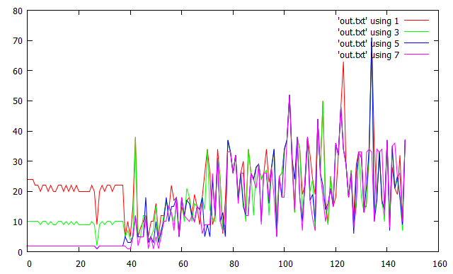
(10/14) so there are 8 different hard seed generation techniques and changing output to be tab separated & graphing columns 7:1 graphs the max nonmono run length versus the starting seed bit size. and there are (8 * 7)/ 2 possible comparisons between two different seed generation methods. comparing all these does not seem to lead to any noticeable “non-constant-bounded” or “consistently increasing” measurements, or “outlier” type differences where one method consistently leads to larger or smaller max nonmono run lengths versus another. by this it is meant the graphs increase in an “early” range of seed bit lengths about 1-~250. then they seem to flatten. caveat though, the results are noisy, not very smooth. they could hopefully be smoothed by aggregating more trajectories than the 500 here (line 182). the max non mono run length encountered is about ~50 for the “z” random method (which of all methods can work with/ generate the largest starting seeds).

(later) changing the trajectory count to 1000, 2000 for the “z” random method leads to similar results as reported earlier with the length-unscaled trajectory integrations. the deviation in the plots does not seem to decrease much, or maybe at all.

(10/16) 💡 ❗ was wondering how that purely local adj6 strategy above would fare wrt the max nonmono run length metric and whipped out some code to analyze it, and results are somewhat surprising, they seem have substantially less deviation than the global strategy (working from memory)! 1^st, a graph analyzing it for some random 10-binary-digit starting seeds, called with ARGV[0]=1. there are 4 modes, based on two modes of log-scale aggregating the “cross-section” of iterates (either integrating the cross-section and then taking the truncated log lines 157-158, or integrating the truncated log lines 154-155), and two modes where the “seen” cache is turned on or off. as in the graph these all have a dramatic effect on the appearance of the trendlines. the log-scale aggregation mode has the biggest effect on shape either smooth/ linear or edgy/ angular and the seen cache logic seems to mostly just compress the total random walk significantly. for larger binary seeds this compression seems to increase significantly.

the 2^nd graph is the graph of the max nonmono run length metric for random seeds of bit size 1-1000 (generation scheme/ARGV[0]=z). the “green” mode seems to do the best and in comparison the other modes seem to have a very-gradual creeping-upward trend advancing rightward. this corresponds to the “edgy” aggregation mode. the integrations are over 100 trajectories (lines 183, 200).

scale3.rb

(10/26) got around to testing the “largest partial integration 1^st” strategy across all the different hard seeds. this is a nice demonstration of the value/ utility of this “test framework”. there are 8 different seed generation algorithms and 4 different integration modes, this code tests all the cases and outputs the max nonmono run length metric sequentially for each different integration mode. the selection strategy noticeably fails for several of the seed generation strategies, most dramatically the 4^th; which turns out to be ‘w’ or the “glide width difference” algorithm. it took ~4hr to generate these graphs. (2020 hindsight/ cosmetic tweak: should have had this code separate the 8 separate runs with larger space gaps.)

scale3b.rb

(10/28) this is a test of a similar local smoothing strategy that “advances” the points in the bunch that have the largest cumulative/ partial integration away from the average and yields similar results. only 1 integration mode was tested. it has some very noticeable large early spikes in the 3^rd and 6^th seed generation strategies (‘m’, ‘c’). as thought of/ mentioned previously the separate strategies are separated by a short (20 width) gap.

scale4.rb