happy 2nd anniversary to this blog! ⭐ ❗ 😎 😀 returning to a theme of collatz reverse tree visualization. a bunch of riffs and some other misc ideas tried out recently. nothing spectacular (in bland contrast to the last flashy-but-semimanic episode) but just posting these partly for archival/ log purposes. (brief related news, got some positive feedback on the subj on mathoverflow.)
these algorithms use more complex comparison metrics, a few quadratic complexity instead of linear complexity, to decide which points to advance next. they exhibit transition-point and tipping-point like behaviors where eg there are two different regimes, one where points are scattered between horizontally increasing lines and one where they line up in “fenceposts” (vertical). (they also fix a defect noted in that earlier code where some additional spurious points (not strictly in the collatz problem) were included.)
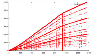
1st, find the nearest point to the prior traversed points. (arg1=5000). this took something like an hour to generate. there is a remarkable phase/regime/slope change at the fencepost for x=~940.
l2 = [2]

seen = {1 => nil}
mx = 0
j = 0

ARGV[0].to_i.times \
{

	z = l2.min_by \
	{
		|x|
		(x - seen.keys.min_by { |y| (y - x).abs }).abs
	}

#	p([z, l2, seen.keys])
	if (z > mx) then
		mx = z
		j += 1
	end
	puts([j, z].join("\t"))
	$stdout.flush
	l2.delete(z)
	seen[z] = nil

	l = [z * 2]
	l << (z - 1) / 3 if (z % 3 == 1 && ((z - 1) / 3).odd?)
	l.each \
	{
		|x|
		next if (seen.member?(x))
		l2 << x
	}
}
next, similar, but nonlinear weighting the x,y coordinates deltas in the next-point ranking/ comparison differently. took hours to generate.
def d(p1, x)

	return 100*(p1[0] - x) ** 2 + (p1[1] - $seen[x]) ** 2

end

l2 = [[2, 0]]

$seen = {1 => 0}
mx = 0
j = 0

ARGV[0].to_i.times \
{

	z = l2.min_by \
	{
		|x|
		d(x, $seen.keys.min_by { |y| d(x, y) })
	}

	z0 = z[0]
	if (z0 > mx) then
		mx = z0
		j += 1
	end
	puts([j, z0].join("\t"))
	$stdout.flush
	l2.delete(z)
	$seen[z0] = mx

	l = [z0 * 2]
	l << (z0 - 1) / 3 if (z0 % 3 == 1 && ((z0 - 1) / 3).odd?)
	l.each \
	{
		|x|
		next if ($seen.member?(x))
		l2 << [x, mx]
	}
}
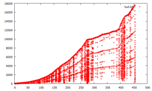
next, a linear time comparison algorithm instead of quadratic, just try to find nearest points to current previously seen point average. this is surprisingly, strikingly nearly identical to plot #1. a strange attractor?
l2 = [2]

seen = {1 => nil}
mx = 0
j = 0

ARGV[0].to_i.times \
{
	a = 0
	seen.keys.each { |x| a += x }
	a = a.to_f / seen.size

	z = l2.min_by \
	{
		|x|
		(x - a).abs
	}

#	p([z, l2, seen.keys])
	if (z > mx) then
		mx = z
		j += 1
	end
	puts([j, z].join("\t"))
	$stdout.flush
	l2.delete(z)
	seen[z] = nil

	l = [z * 2]
	l << (z - 1) / 3 if (z % 3 == 1 && ((z - 1) / 3).odd?)
	l.each \
	{
		|x|
		next if (seen.member?(x))
		l2 << x
	}
}
next, this code attempts to balance out by selecting new points in the “midpoints” of the prior point cloud, where there are the largest gaps. again a quadratic time algorithm.
l2 = [2]

seen = {1 => nil}
mx = 0
j = 0

ARGV[0].to_i.times \
{
	l = seen.keys.sort

	m = 0
	z = nil
	l2.each \
	{
		|x|
		i = 0
		i += 1 while (i < l.size && x > l[i])
		next if (i == l.size)
		a = i > 0 ? l[i - 1] : 0
		b = l[i]
		r = (x - a) * (b - x)
		z, m = x, r if (r > m)
	}


	if (z.nil?) then
		z = l2.min
		j += 1
	end
	puts([j, z].join("\t"))
	$stdout.flush
	l2.delete(z)
	seen[z] = nil

	l = [z * 2]
	l << (z - 1) / 3 if (z % 3 == 1 && ((z - 1) / 3).odd?)
	l.each \
	{
		|x|
		next if (seen.member?(x))
		l2 << x
	}
}
its remarkable that very different adaptive algorithms lead to the overall same output structure, suggesting some kind of resilience or strange attractor. there are small differences in the output ordering of points but the algorithms converge to similar overall structures. and getting nearly identical results with the linear vs quadratic measurement is also surprising.
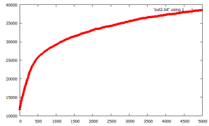
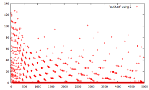
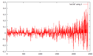
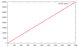
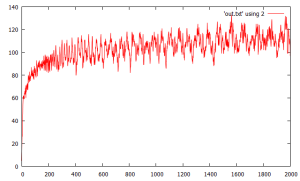
next, this seems like a notable finding. this is similar to an earlier idea of using a fixed-sized “relatively small” running buffer (200 points) and extracting min points from the buffer. the semi surprising finding is that the total buffer integration is orderly monotonically increasing. 2nd graph shows deltas between adjacent curve points.
def f(n)


	c = 0
	while (n != 1)
		n = n.even? ? n / 2 : n * 3 + 1
		c += 1
	end

	return c
end


l = []

n = 3
t = 0
w = 200
t2 = nil
(w + 5000).times \
{
	x = f(n)
	l << x
	t += x
	if (l.size > w) then
		i = (0...l.size).min_by { |j| l[j] }
		t -= l[i]
		l.delete_at(i)
		puts([t, t - t2].join("\t")) if (!t2.nil?)
		t2 = t
	end
	n += 2
}
its also naturally worth looking at the “age” of points removed from the buffer.
def f(n)


	c = 0
	while (n != 1)
		n = n.even? ? n / 2 : n * 3 + 1
		c += 1
	end

	return c
end


l = []

n = 3
t = 0
w = 200
t2 = nil
a = 0
m = 20000
(w + m).times \
{
	x = f(n)
	l << [x, n]
	t += x
	if (l.size > w) then
		i = (0...l.size).min_by { |j| l[j] }
		p = l[i][1]
		t -= l[i][0]
		l.delete_at(i)
		puts([t, n - p, t - t2].join("\t")) if (!t2.nil? && a > m - 10000)
		t2 = t
	end
	n += 2
	a += 1
}
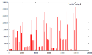
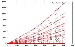
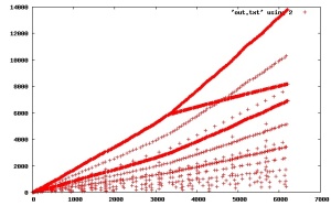
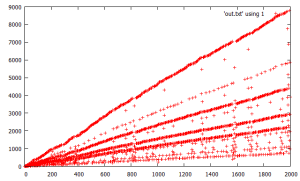
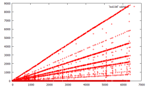
(10/25) this following simple code uses a 1000 point buffer and iterates forward through the smallest element, and replaces it with the next sequential unexplored/ unterminated integer if its trajectory reaches 1. the 1st graph is the new points added to the buffer and the 2nd graph is the “resolved” points, where gaps in the 1st correspond to no new point(s) added during that iteration and the buffer processed (smallest element advanced). the algorithm outputs resolved points in batches as new unverified trajectories “hit/touch” the verified trajectories; this is roughly the same as trajectory merge logic described earlier. the 2nd graph is notable in that “higher” points are very regular in their spacing/ alignment and the plot gets more random/ scattered as moving to “lower” points. it also shows a notable/ major regime change around x=~3200 seen in in the top line slope change and “fork/ bifurcation” and also coinciding/ corresponding with a prior gap in the first graph.
#!/usr/bin/ruby1.8


l = []

seen = {}
done = {1 => nil}


n = -1
1000.times \
{
        n += 4

        seen[n] = l.size
        l << [n]
}

5000.times \
{
        i = -1
        l2 = l.map { |l1| [l1[-1], i += 1] }

        n2, i = l2.min
        puts([0, n2].join("\t"))

        n2 = (n2 % 2 == 0) ? n2 / 2 : n2 * 3 + 1
        if (done.member?(n2)) then
                l[i].each { |x| done[x] = nil; p(x) }
                l[i] = [n += 4]
        end

        if (!(j = seen[n2]).nil?)

                x = l[j][-1]
                l[j] |= l[i]
                l[j] << x
                l[i] = [n += 4]
                seen[n] = i
        else
                l[i] << n2
                seen[n2] = i
        end

}
(10/28) returning to another idea touched on earlier. those experiments showed an apparently level (constant bounded?) vertex count of blockwise-piece graphs even for very high trajectories. based on a remarkable property associated with transducer constructions of TMs, if any TM can be constructed that resolves all values of the problem (or any other problem) in a constant number of iterations, that is provable within the transducer framework. the details are somewhat involved but not actually very complex.
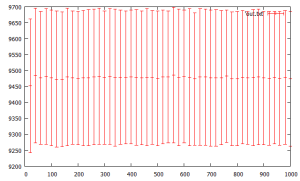
however, presumably these graphs are misleading. from an earlier experiment (end of the same post), apparently arbitrarily long sequences/ trajectories exist, although not so sure how to prove this. they might be or seem to be hidden “outside” the monte carlo samples like (very rare?) needles buried in the haystack. anyway with that caveat, here is another experiment surveying the haystack up to large initial trajectories and showing the standard deviation error bars. the “apparently constant property” is visible, but this maybe also shows/ demonstrates the limitations of visualizations, and the limitations of aggregate statistics (averages) esp with non-gaussian & fractal distributions (popularized by Nassem Taleb as the so-called “black swan” phenomenon). this randomly samples the space up to with 5000 samples at each interval, each 1000 trajectory blockwise piece graphs and shows no discernable slope.
def f(n)


	n2 = n
	while (n2 >= n)

		n2 = n2.even? ? n2 / 2 : n2 * 3 + 1
		break if ($seen.member?(n2))
		$seen[n2] = nil

	end


end

def sample(n, c, w)


	t = t2 = 0
	c.times \
	{

		m = 2 ** n + rand(2 ** n) | 1
		$seen = {}
		w.times \
		{
			f(m)
			m += 2
		}
		x = $seen.size
		t += x
		t2 += x**2
	}
	a = t.to_f / c
	return a, Math.sqrt(t2.to_f / c - a ** 2)
end


n = 20
50.times \
{
	a, sd = sample(n, 5000, 1000)
	puts([n, a, sd].join("\t"))
	$stdout.flush
	n += 20
}
(10/31) revisiting the “valid suffix/prefix enumeration” code. (recall) this code looks at binary suffixes for initial seeds that dont “fall below” and recursively generates them. an interesting factoid is that this tree always has at least one (min) or two branches (max) at each node, never zero. it lists the source prefix and then the 1 or 2 new branching prefixes as indented. not sure how to prove this at the moment. it seems to have something to do with prefixes being in the form . this also does a histogram of ‘1’s found in the binary prefixes, they seem to be somewhat smoothly or normally distributed. ARG[0] = 10
def check(n, b)

	a = n
	b0 = b
        while (a >= n)

            if (b.odd?) then
		a *= 3
		b = b * 3 + 1
            end
		if (b.even?) then
			if (!a.even?) then
				return [b0]
			end
			a /= 2
			b /= 2
		end
	end

	return []

end


def scan(p)

    n = 2**p
    l = []

    (1...n).each \
    {
        |i|

	l += check(n, i)

        a = n
        b = i
     }

	return l
end

def wrap(p, x, n)

	l = check(2 ** p, x)
	return [] if (l.empty?)
	puts("\t"+sprintf("%0#{p}d", l[0].to_s(2)).reverse)
	return l
end

def recur(n)

	l = [1]

	(2..n).each \
	{
		|p|
		l2 = []
		l.each \
		{
			|x|
			puts(sprintf("%0#{p - 1}d", x.to_s(2)).reverse)
			l2 += wrap(p, x, n)
			l2 += wrap(p, x + (2 ** (p - 1)), n)
		}
		puts("---")
		l = l2
	}
	return l
end


n = ARGV[0].to_i

l2 = recur(n)

h = {}
l2.each \
{
	|x|
	c = x.to_s(2).split('').select { |y| y == '1' }.size
	h[c] = 0 if (h[c].nil?)
	h[c] += 1
}
p(h)
1
	11
---
11
	110
	111
---
110
	1101
111
	1110
	1111
---
1101
	11011
1110
	11100
1111
	11110
	11111
---
11011
	110110
	110111
11100
	111000
	111001
11110
	111100
	111101
11111
	111110
	111111
---
110110
	1101100
	1101101
110111
	1101111
111000
	1110001
111001
	1110010
	1110011
111100
	1111001
111101
	1111010
	1111011
111110
	1111100
	1111101
111111
	1111110
	1111111
---
1101100
	11011000
	11011001
1101101
	11011010
1101111
	11011111
1110001
	11100010
1110010
	11100101
1110011
	11100110
	11100111
1111001
	11110011
1111010
	11110100
1111011
	11110110
	11110111
1111100
	11111000
	11111001
1111101
	11111011
1111110
	11111100
	11111101
1111111
	11111110
	11111111
---
11011000
	110110000
	110110001
11011001
	110110010
	110110011
11011010
	110110100
	110110101
11011111
	110111110
	110111111
11100010
	111000100
	111000101
11100101
	111001010
	111001011
11100110
	111001100
	111001101
11100111
	111001110
	111001111
11110011
	111100110
	111100111
11110100
	111101000
	111101001
11110110
	111101100
	111101101
11110111
	111101110
	111101111
11111000
	111110000
	111110001
11111001
	111110010
	111110011
11111011
	111110110
	111110111
11111100
	111111000
	111111001
11111101
	111111010
	111111011
11111110
	111111100
	111111101
11111111
	111111110
	111111111
---
110110000
	1101100000
	1101100001
110110001
	1101100010
	1101100011
110110010
	1101100100
	1101100101
110110011
	1101100110
110110100
	1101101000
	1101101001
110110101
	1101101011
110111110
	1101111100
	1101111101
110111111
	1101111111
111000100
	1110001000
111000101
	1110001010
	1110001011
111001010
	1110010100
	1110010101
111001011
	1110010111
111001100
	1110011000
	1110011001
111001101
	1110011010
	1110011011
111001110
	1110011100
	1110011101
111001111
	1110011110
111100110
	1111001100
	1111001101
111100111
	1111001110
111101000
	1111010000
	1111010001
111101001
	1111010010
111101100
	1111011000
	1111011001
111101101
	1111011011
111101110
	1111011100
	1111011101
111101111
	1111011110
	1111011111
111110000
	1111100000
	1111100001
111110001
	1111100011
111110010
	1111100100
	1111100101
111110011
	1111100110
	1111100111
111110110
	1111101100
111110111
	1111101110
	1111101111
111111000
	1111110000
111111001
	1111110010
	1111110011
111111010
	1111110100
	1111110101
111111011
	1111110110
	1111110111
111111100
	1111111000
	1111111001
111111101
	1111111010
	1111111011
111111110
	1111111100
	1111111101
111111111
	1111111110
	1111111111
---
{4=>2, 5=>9, 6=>16, 7=>17, 8=>12, 9=>7, 10=>1}
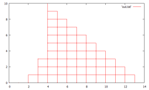
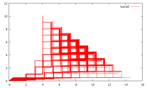
this is some funky code that visualizes the prefixes using a simple random walk-like approach & shows how it is constrained/ confined in a remarkable stairstep pattern, and also helps to show/ understand how the 1’s are ordered/ distributed inside the binary expansion. (has a sort of zen-like simplicity eh?) 😎 the 2nd graph uncomments the offsetting feature/ line. ARGV[0] = 14
def check(n, b)

	a = n
	b0 = b
        while (a >= n)

            if (b.odd?) then
		a *= 3
		b = b * 3 + 1
            end
		if (b.even?) then
			if (!a.even?) then
				return [b0]
			end
			a /= 2
			b /= 2
		end
	end

	return []

end


def scan(p)

    n = 2**p
    l = []

    (1...n).each \
    {
        |i|

	l += check(n, i)

        a = n
        b = i
     }

	return l
end

def wrap(p, x, n)

	l = check(2 ** p, x)
	return [] if (l.empty?)
#	puts("\t"+sprintf("%0#{p}d", l[0].to_s(2)).reverse)
	return l
end

def recur(n)

	l = [1]

	(2..n).each \
	{
		|p|
		l2 = []
		l.each \
		{
			|x|
#			puts(sprintf("%0#{p - 1}d", x.to_s(2)).reverse)
			l2 += wrap(p, x, n)
			l2 += wrap(p, x + (2 ** (p - 1)), n)
		}
#		puts
		l = l2
	}
	return l
end


n = ARGV[0].to_i

l2 = recur(n)

l2.each_with_index \
{
	|x, i|
	s = sprintf("%0#{n}d", x.to_s(2)).reverse
	x = y = 0 #i * 0.0007
	s.split('').each \
	{
		|b|
		puts([x, y].join("\t"))
		b == '1' ? x += 1 : y += 1
		puts([x, y].join("\t"))
		puts
	}
}
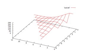
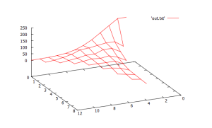
another natural/ nice way of visualizing these results is a 3d “surface plot histogram”, 2 perspective angles below. here point height is the histogram count and (x, y) is the intermediate location/ visits of the walks. using this method, the starting location (0,0) has the highest count and counts decrease from there. this also highlights the smoothness of the distribution. another obvious idea is to just graph the counts of ending locations.
def check(n, b)

	a = n
	b0 = b
        while (a >= n)

            if (b.odd?) then
		a *= 3
		b = b * 3 + 1
            end
		if (b.even?) then
			if (!a.even?) then
				return [b0]
			end
			a /= 2
			b /= 2
		end
	end

	return []

end


def scan(p)

    n = 2**p
    l = []

    (1...n).each \
    {
        |i|

	l += check(n, i)

        a = n
        b = i
     }

	return l
end

def wrap(p, x, n)

	l = check(2 ** p, x)
	return [] if (l.empty?)
#	puts("\t"+sprintf("%0#{p}d", l[0].to_s(2)).reverse)
	return l
end

def recur(n)

	l = [1]

	(2..n).each \
	{
		|p|
		l2 = []
		l.each \
		{
			|x|
#			puts(sprintf("%0#{p - 1}d", x.to_s(2)).reverse)
			l2 += wrap(p, x, n)
			l2 += wrap(p, x + (2 ** (p - 1)), n)
		}
#		puts
		l = l2
	}
	return l
end


n = ARGV[0].to_i

l2 = recur(n)

h = {}
l2.each_with_index \
{
	|x, i|
	s = sprintf("%0#{n}d", x.to_s(2)).reverse
	x = y = 0
	s.split('').each \
	{
		|b|
		b == '1' ? x += 1 : y += 1
		z = [x, y]
		h[z] = 0 if (h[z].nil?)
		h[z] += 1
	}
}

def fmt(p, h)

	return (p + [h[p]]).join("\t")
end

h.sort.each \
{
	|p0, z|

	p1 = [p0[0] + 1, p0[1]]
	p2 = [p0[0], p0[1] + 1]

	[p1, p2].each \
	{
		|p|
		printf("%s\n%s\n\n\n", fmt(p0, h), fmt(p, h)) if (h.member?(p))
	}

}
(11/4) heres another idea where trajectories are resolved in parallel, working from min elements in the trajectory frontiers, but not by ending at 1 and instead resolved at the “fall below” point. it uses a “reverse-directed” graph/tree of the trajectories to mark resolved points and again a typical “seen” cache to recognize previously visited/ processed points. the “mark” subroutine is a breadth-1st reverse/ backward traversal of an “in flight” trajectory converted to “resolved”. the 2nd plot is with the commented line uncommented and puts in “zero” points for loop iterations where new trajectories are started. it leads to a more ordered/ linear plot.
def mark(n)

	l = [n]
	while (!l.empty?)

		n = l.shift
		next if ($seen.member?(n))
		$c += 1
		p(n)
		$seen[n] = nil
		l.push(*$back[n].keys) if ($back.member?(n))

	end

end

at = {1 => 1}
m = 3
$back = {}
$seen = {}
$c = 0

loop \
{
	l = at.to_a.min

	if (l.nil? || m < l[0]) then
		a = n = m
		m += 2
#		puts([0, n].join("\t"))
	else
		n, a = l
		at.delete(n)
	end

	n2 = n.even? ? n / 2 : n * 3 + 1
	$back[n2] = {} if ($back[n2].nil?)
	$back[n2][n] = nil

	if (n2 > a)
		at[n2] = at[n2].nil? ? a : [a, at[n2]].min
	else
		mark(n2)
	end

	break if ($c == 2000)
}
(11/7) this is a natural question about how a depth first versus a breadth first search of prefix enumeration leads to larger trajectories. the idea is to mix some breadth exploration with the depth-first exploration. the output in (a, b, c, d) format shows that about 10 breadth iterations per depth iteration leads to about 30% longer trajectories (column a) at the cost of a larger frontier set, but the “gain” mostly flattens/ plateaus out after that. b is the size of the starting seed in bits, c is the size of the frontier set, and d is the iteration.
def count(n)
	c = 0
	while (n != 1)
		n = n.even? ? n / 2 : n * 3 + 1
		c += 1
	end
	return c
end


def check(p, b)

	n = 2 ** p
	a = n
	b0 = b
	c = 0
        while (a >= n)

		if (b.odd?) then
			a *= 3
			b = b * 3 + 1
		else
			return [[b0, c + count(b), p + 1]] if (!a.even?)
			a /= 2
			b /= 2
		end
		c += 1
	end

	return []

end


def recur3(m, j)

	l = [[1, 0, 2]]
	t = 0

	loop \
	{
		l.sort_by! { |x, c, p| -c }

		t += 1
		break if (t >= m)
		j.times \
		{
			x, c, p = l.shift

			l += check(p, x)
			l += check(p, x + (2 ** (p - 1)))
		}
	}
	p(l[0][1..2] + [l.size, j])
	return l
end

m = 150
(1..20).each { |j| l2 = recur3(m, j) }
[1401, 133, 128, 1]
[1443, 146, 257, 2]
[1935, 153, 417, 3]
[1691, 146, 517, 4]
[1879, 155, 720, 5]
[1860, 155, 852, 6]
[2049, 154, 992, 7]
[1863, 156, 1115, 8]
[1821, 155, 1297, 9]
[1979, 155, 1424, 10]
[1814, 156, 1542, 11]
[1902, 156, 1708, 12]
[2100, 157, 1892, 13]
[2100, 157, 2034, 14]
[2100, 157, 2183, 15]
[1998, 157, 2330, 16]
[2100, 157, 2460, 17]
[2142, 157, 2638, 18]
[1774, 157, 2710, 19]
[2009, 158, 2911, 20]
this code looks at the density of 1s in the binary expansion of trajectory points for a long 200 “depth” trajectory (length 2439 iterations). it reminds me of research onto the “knife edge” point of satisfiability. it shows that long trajectories apparently have a fractal-like self similar structure where density of 1s in iterates tends to hover around 50%, and the divergence/ deviation tends to widen at the end.
there is an interesting way to view/ interpret this in terms of complexity “hardness” with more parallels to the SAT knife edge. the time to resolve the trajectory is like the complexity of the algorithm. an instance is recursively resolved. if the next instance is self-similar to the previous instance (iterate), hardness is maximized.
def count(n)
	c = 0
	while (n != 1)
		n = n.even? ? n / 2 : n * 3 + 1
		c += 1
	end
	return c
end


def check(p, b)

	n = 2 ** p
	a = n
	b0 = b
	c = 0
        while (a >= n)

		if (b.odd?) then
			a *= 3
			b = b * 3 + 1
		else
			return [[b0, c + count(b), p + 1]] if (!a.even?)
			a /= 2
			b /= 2
		end
		c += 1
	end

	return []

end


def recur3(m, j)

	l = [[1, 0, 2]]
	t = 0

	loop \
	{
		l.sort_by! { |x, c, p| -c }

		t += 1
		break if (t >= m)
		j.times \
		{
			x, c, p = l.shift

			l += check(p, x)
			l += check(p, x + (2 ** (p - 1)))
		}
	}
	return l[0][0]
end

def density(n)

	while (n != 1)

		n = n.even? ? n / 2 : n * 3 + 1
		c = 0
		s = n.to_s(2)
		s.split('').each { |x| c += x.to_i }
		puts([Math.log(n), c.to_f / s.length - 0.5].join("\t"))
	end

end

n = recur3(200, 10)
density(n)
(11/19) this is some straightforward code that achieves a very nice balance of outputting resolved trajectory seeds in an almost linear fashion with a slowly increasing buffer size. it simply advances a large buffer of current trajectories each in parallel and always adds the current iterate to the (end of the) buffer. it has no logic to deal with previously seen iterates. there is a little extra logic to look at the last trend versus the output summarized overall trend. 1st graph is the resolved seeds and second is the buffer size.
def f(x)

	x = x.even? ? x / 2 : x * 3 + 1
end

l = []
l3 = []
l4 = []
c = 2000
m = 20000
d = m.to_f / c

n = 3
m.times \
{
	|j|
	l << [n]
	n += 2
	i = 0
	while (i < l.size)

		l[i] << f(l[i][-1])
		if (l[i][-1] == 1) then
			l2 = l.delete_at(i)
			l3 << [l2[0], l.size]
			l4 << l3[-1] if (l4.size < j / d)

			l3.shift if (l3.size > c)
			next
		end
		i += 1

	end

}
#p(l4.size)
l4.each { |x| puts(x.join("\t")) }
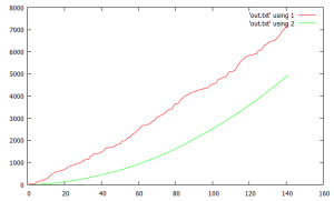
another quick idea reminiscent of an earlier one. this code sequentially accumulates trajectory lengths in a way that enforces a “minimally” monotonically increasing trend (red). it tracks which seeds cross new maximum boundaries. this results in a very orderly graph of the 2nd statistic (green).
def f(n)


	c = 0
	while (n != 1)
		n = n.even? ? n / 2 : n * 3 + 1
		c += 1
	end
	return c
end

m = 1
m2 = 0

n = 3
5000.times \
{
	|j|

	m2 += f(n)
	if (m2 > m) then
		m = m2
		m2 = 0
		puts([m, j].join("\t"))
	end

	n += 2
}


Pingback: Collatz, striking visualization of binary density for 3x + 1 operation! | Turing Machine
Pingback: ***startling*** collatz plateau! | Turing Machine